Numerical and graphical methods of solving equations

After studying this section, you will be able to:

• solve equations that cannot be solved with simple manipulative methods by using systematic trial and improvement in various forms
• solve equations that cannot be solved with simple manipulative methods by using graphical methods

Trial and Improvement

Sometimes it may not be possible to solve an equation using simple algebra, for example x³ + 2x² − 5 = 0. However, there are approximate methods that can be refined to give solutions to any degree of accuracy. The two most important approaches involve trial and improvement and graphical methods.

Image

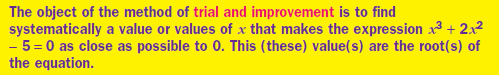
NOTE:The trials are chosen for a reason, not haphazardly.

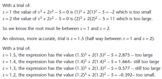
Image

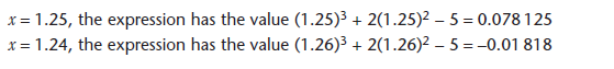
NOTE:

The root lies between x = 1.24 and 1.25

By choosing x = 1.245 we can find whether x = 1.24 or x = 1.25 is closer

Image

Image

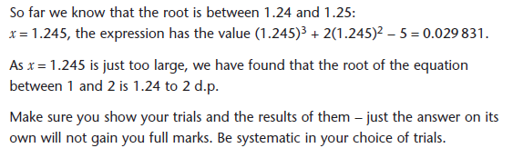
NOTE:Greater accuracy can be achieved by continuing the process. A sensible next value to try would be x = 1.244.

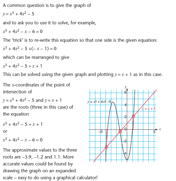
Graphical methods to solve equations

NOTE:In some cases the graph will be drawn for you, but you still need to be able to draw graphs like this.

Image

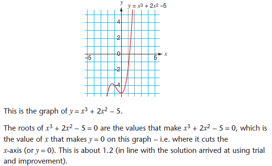
We know that the solution to two simultaneous equations is the coordinates of the point of intersection of the two equations drawn as straight lines or curves.

Image

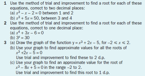
PROGRESS TEST

Image

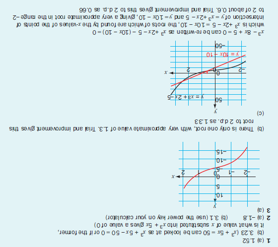
PROGRESS TEST ANSWERS

Image